Ce cours d’arithmétique est conforme au programme des filières MPSI et MP2I. Il contient des exemples et des exercices d’application qui faciliteront votre assimilation du contenu. N’hésitez pas à consulter notre série d’exercices corrigés pour acquérir une maîtrise solide du cours.
Définition 1 : Soient a et b deux entiers relatifs. On dit que a divise b lorsque : \exists c \in \mathbb{Z}, \ b=ac . On note dans ce cas a | b et on dit que a est un diviseur de b et que b est un multiple de a. On note D(b) l’ensemble des diviseur de b et a \mathbb{Z} l’ensemble des multiples de a.
Proposition 1 : Soient a,b,c,d \in \mathbb{Z}. i) a | b\text{ et } c | d \Rightarrow a c| b d . ii) a | b et a|c \Rightarrow \forall \lambda, \mu \in \mathbb{Z}, \ a| \lambda b+\mu c. iii) a | b et b|c \Rightarrow a| c. iv) a | b et b|a \Rightarrow | a|=| b | . v) a|b \Rightarrow a| b c. vi) a b|c \Rightarrow a| c et b | c.
Démonstration : i) On suppose que a | b\text{ et } c | d. Donc \exists k_{1}, k_{2} \in \mathbb{Z}, \ b=k_{1} a et d=k_{2} c. Par produit b d=\left(k_{1} k_{2}\right) a c. Donc a c | b d.
Théorème de la division euclidienne : \forall(a, b) \in \mathbb{Z} \times \mathbb{N}^{*}, \exists !(q, r) \in \mathbb{Z} \times \llbracket 0, b-1 \rrbracket, \quad a=q b+r . q est dit quotient de la division euclidienne de a par b. r est dit reste de la division euclidienne de a par b.
Démonstration : On va utiliser un raisonnement par analyse-synthèse. Soit (a, b) \in \mathbb{Z} \times \mathbb{N}^{*}. Analyse : On suppose qu’il existe (q, r) \in \mathbb{Z} \times \llbracket 0, b-1 \rrbracket, \ a=q b+r. Donc \frac{a}{b}=q+\frac{r}{b}. En utilisant la partie entière \left\lfloor\frac{a}{b}\right\rfloor=q+\left\lfloor\frac{r}{b}\right\rfloor=q. Ainsi r=a-q b=a-b\left\lfloor\frac{a}{b}\right\rfloor. Au passage nous avons montré l’unicité de q et r sous-réserve d’existence. Synthèse : On pose q=\left\lfloor\frac{a}{b}\right\rfloor et r=a-b q. On a q, r \in \mathbb{Z} et a=b q+r. Par définition de la partie entière q \leqslant \frac{a}{b}<q+1. Donc bq \leqslant a<b q+b ce qui nous donne 0 \leqslant r<b. Et finalement r \in \llbracket 0, b-1 \rrbracket. Conclusion : On vient de démontrer le théorème de la division euclidienne en utilisant le raisonnement par analyse-synthèse.
Exemple 2 : 13=2 \times 5+3 est la division euclidienne de 13 par 5. 2 et 3 sont respectivement le quotient et le reste de la division euclidienne de 13 par 5.
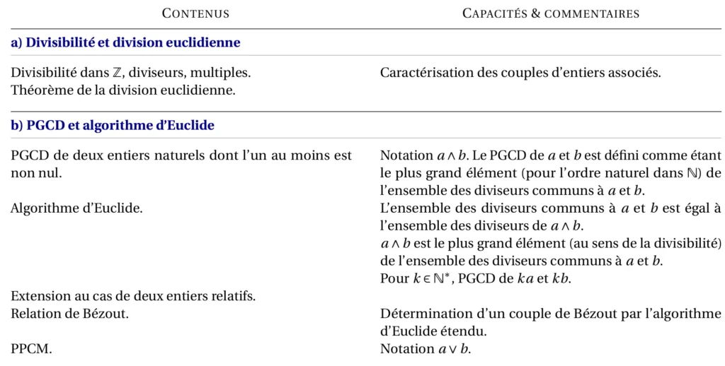
II) PGCD et algorithme d’Euclide
Proposition-définition (PGCD de deux entiers): Soient (a, b) \in \mathbb{Z}^{2} \setminus \{(0,0)\}. L’ensemble D(a) \cap D(b) admet un plus grand élément qu’on appelle le plus grand commun diviseur de a et b. On le note a \wedge b ou \operatorname{PGCD}(a, b). On convient que 0 \wedge 0=0.
Justification : D(a) \cap D(b) est une partie de \mathbb{Z} non vide (car contient 1 ) et majorée (par \max (|a|,|b|), donc admet un plus grand élément.
Démonstration : i) On va montrer l’égalité de ces deux ensembles par une double inclusion « \subset » Soit d \in D(a) \cap D(b). On a d \in D(a) et d \in D(b) donc d | a et d | b. D’où d | a-b q c’est-à-dire d | r ou d’une façon équivalente d \in D(r). On vient de montrer que D(a) \cap D(b) \subset D(b) \cap D(\mathrm{r}). « \supset » Soit d \in D(b) \cap D(\mathrm{r}). On a d \in D(b) et d \in D(\Omega) ce qui se traduit par d | b et d | \mathrm{r}. Ainsi d | b q+\mathrm{r} d’où d | a c’est-à-dire d \in D(a). Donc d \in D(a) \cap D(b). On vient de montrer que D(b) \cap D(r) \subset D(a) \cap D(b). On Conclut alors que D(a) \cap D(b)=D(b) \cap D(r). ii) Montrons que a \wedge b=b \wedge \mathrm{r}. 1^{\text {er }} \text { cas : Si } b=0 : Alors r=a et par la suite a \wedge b=b \wedge r . 2^{\text {ème }} \text { cas : Si } b \neq 0 . Alors a \wedge b=\max (D(a) \cap D(b))=\max (D(b) \cap D(r))=b \wedge \mathrm{r} .
Exercice d’application 1 : Soient a et m deux entiers tels que a \geqslant 3 et m \geqslant 2. 1) Déternimer q_{m} le quotient de la division euclidienne de a^{m} par a-1. 2) Montrer que q_{m} \wedge(a-1)=m \wedge(a-1).
Corrigé : 1) On a a^{m}-1=(a-1) \sum\limits_{k=0}^{m-1} a^{k}. Donc a^{m}=(a-1) \sum\limits_{k=0}^{m-1} a^{k}+1. Puisque 0 \leqslant 1<a-1, alors 1 est le reste de la division euclidienne de a^{m} par a-1 et q_{m}=\sum\limits_{k=0}^{m-1} a^{k} est le quotient de cette division. 2) q_{m}=\sum\limits_{k=0}^{m-1} a^{k}=\sum\limits_{k=0}^{m-1}\left((a-1) \sum\limits_{j=0}^{k-1} a^{j}+1\right)=(a-1) \sum\limits_{k=0}^{m-1} \sum\limits_{j=0}^{k-1} a^{j}+m. Donc q_{m} \wedge(a-1)=(a-1) \wedge m.
Proposition 3 : \forall a, b \in \mathbb{Z}, \ D(a) \cap D(b)=D(a \wedge b). Autrement dit : \forall a, b \in \mathbb{Z}, \forall d \in \mathbb{Z}, \quad d | a \text{ et } d|b \Leftrightarrow d| a \wedge b.
Démonstration : Montrons d’abord par récurrence forte que \forall a \in \mathbb{N}, \forall b \in \mathbb{Z}, D(a) \cap D(b)=D(a \wedge b). Pour \bullet \ a=0. D(a)=\mathbb{Z} et a \wedge b=|b|. Donc D(a \wedge b)=D(|b|)=D(b)=D(a) \cap D(b). \bullet Soit a \in \mathbb{N}. On suppose que \forall k \in \llbracket 0, a \rrbracket, \forall b \in \mathbb{Z}, D(k) \cap D(b)=D(k \wedge b). Soit b \in \mathbb{Z}, par division euclidienne de b par a+1 il existe (q, r) \in \mathbb{Z} \times \llbracket 0, a \rrbracket, b=q(a+1)+r. Il résulte de cette égalité D(a+1 \wedge b)=D(a+1 \wedge r). Par l’hypothèse de la récurrence forte appliquée sur r on obtient D(a+1 \wedge b)=D(a+1) \cap D(r). Donc D(a+1 \wedge b)=D(a+1) \cap D(b). \bullet On conclut par le principe de la récurrence forte que \forall a \in \mathbb{N}, \forall b \in \mathbb{Z}, D(a) \cap D(b)=D(a \wedge b).
Généralisons maintenant ce résultat sur \mathbb{Z}. Soient a \in \mathbb{Z}^{-}et b \in \mathbb{Z}. On sait que D(a) \cap D(b)=D(-a) \cap D(b). On a -a \in \mathbb{N} donc par ce qui précède D(a) \cap D(b)=D((-a) \wedge b)=D(a \wedge b).
Algorithme d’Euclide : Soit (a, b) \in \mathbb{Z}^{2}. On pose r_{0}=\max (|a|,|b|) et r_{1}=\min (|a|,|b|). Si \mathrm{r}_{0}=0 \quad Alors a \wedge b=0 Sinon r_{0} \neq 0 \quad Pour k \geqslant 1 \quad \quad Tant que r_{k} \neq 0 \quad \quad \quad On note r_{k+1} le reste de la division euclidienne de r_{k-1} par r_{k}. \quad \quadIl existe N \in \mathbb{N} tel que \mathrm{r}_{N} \neq 0 et r_{N+1}=0 ( \mathrm{r}_{N} est le dernier reste mon nulle dans ces divisions euclidiennes successives). On a alors r_{N}=\operatorname{PGCD}(a, b).
Exemple 4 : Déterminer u, v \in \mathbb{Z} tels que 150 u+54 v=6. L’algorithme d’Euclide fourni une relation de Bézout, on va donc utiliser les calculs de l’exercice d’application 2. 6=42-3 \times 12 6=42-3(54-42) 6=4 \times 42-3 \times 54 6=4 \times(150-2 \times 54)-3 \times 54 6=4 \times 150-11 \times 54
Remarque 1 : i) Les coefficients u, v ne sont pas uniques comme le montre l’exemple : 3=2 \times 2-1 \\ 3=5 \times 1-2. ii) La réciproque de la relation de Bézout est fausse, voici un contre-exemple : 6=6 \times 6-2 \times 15 mais 6 \wedge 15 \neq 6.
Proposition-définition : Soient a\text{ et }b deux entiers non nuls. L’ensemble a \mathbb{Z} \cap b \mathbb{Z} \cap \mathbb{N}^{*} admet un plus petit élément qu’on appelle plus petit commun multiple de a et b. On note \operatorname{PPCM}(a, b)=a \vee b=\min \left(a \mathbb{Z} \cap b \mathbb{Z} \cap \mathbb{N}^{*}\right). On convient que \forall n \in \mathbb{Z}, \ \operatorname{PPCM}(n, 0)=0.
Démonstration : a \mathbb{Z} \cap b \mathbb{Z} \cap \mathbb{N}^{*} est une partie mon vide (car contient |a b| ) de \mathbb{N} donc admet un plus petit élément, ce qui justifie la définition du PPCM.
Proposition 4 : \forall a, b \in \mathbb{Z}, \ a \mathbb{Z} \cap b \mathbb{Z}=PPCM(a, b) \mathbb{Z}. Autrement dit : \forall a, b \in \mathbb{Z}, \forall m \in \mathbb{Z}, \quad a | m \text{ et } b|m \Leftrightarrow \operatorname{PPCM}(a, b)| m.
Démonstration : 1^{ \text{er}} cas : Si a=0 ou b=0. Alors a \vee b=0 et (a \mathbb{Z}=\{0\} ou b \mathbb{Z}=\{0\}). Donc a \mathbb{Z} \cap b \mathbb{Z}=\{0\}=(\mathrm{a} \vee \mathrm{b}) \mathbb{Z}. 2^{\text {ème }} cas : Si a \neq 0 et b \neq 0. Soit m \in \mathbb{Z}. « \Rightarrow » On suppose que a | m et b | m. Par la division euclidienne de m par a \vee b, \exists !(q, r) \in \mathbb{Z} \times \llbracket 0, a \vee b-1 \rrbracket, m=q(a \vee b)+r. On constate que r est un multiple commun de a et b, et puisque r \in \llbracket 0, a \vee b-1 \rrbracket nécessairement r=0. Donc a \vee b | m. « \Leftarrow » On suppose que a \vee b | m. On a a | a \vee b donc par transitivité a | m. Et on a b | a \vee b donc par transitivité b | m.
Démonstration : i) On applique l’algorithme d’Euclide au couple (a, b). En multipliant par |\lambda| toutes les égalités issues de cet algorithme, on obtient l’algorithme d’Euclide du couple (|\lambda| a,|\lambda| b). Donc \operatorname{PGCD}(|\lambda| a,|\lambda| b)=|\lambda| \operatorname{PGCD}(a, b). Ainsi \operatorname{PGCD}(\lambda a, \lambda b)=|\lambda| \operatorname{PGCD}(a, b).
ii) |\lambda| \operatorname{PPCM}(a, b) \mathbb{Z}=|\lambda|(a \mathbb{Z} \cap b \mathbb{Z})=|\lambda| a \mathbb{Z} \cap|\lambda| b \mathbb{Z}=\operatorname{PPCM}(|\lambda| a,|\lambda| b) \mathbb{Z}. On a donc \operatorname{PPCM}(\lambda a, \lambda b)=\operatorname{PPCM}(|\lambda| a,|\lambda| b)=|\lambda| \operatorname{PPCM}(a, b).
Démonstration : 1^{\text{e r}} cas : Si a=0 ou b=0 Alors \operatorname{PGCD}(a, b) \cdot \operatorname{PPCM}(a, b)=0=|a b|. 2^{\text {ème }} cas : si a \neq 0 et b \neq 0 On pose d=\operatorname{PGCD}(a, b) et m=\operatorname{PPCM}(a, b). \exists a, a^{\prime} \in \mathbb{Z}, \quad a=d a^{\prime} et b=d b^{\prime}. On pose \mu=d a^{\prime} b^{\prime}=a^{\prime} b=a b^{\prime}. Alors a | \mu et b | \mu donc m | \mu donc m d | \mu d. C’est-à-dire m d | a b (*). On a : a b \in a \mathbb{Z} \cap b \mathbb{Z}=m \mathbb{Z}. Donc \exists k \in \mathbb{Z}, a b=m k. Or m \in a \mathbb{Z} donc \exists k^{\prime} \in \mathbb{Z}, m=a k^{\prime}. Donc a b=a k k^{\prime} et par la suite b=k \cdot k^{\prime}. Ainsi k | b. Puisque a et b jouent des rôles symétriques alors k | a. Donc k | d donc m k | m d. C’est-à-dire a b | m d (**)|. Par (*) et (**), on conclut que m d=|m d|=|a b|.
Définition 2 : Soient a et b deux entiers relatifs. On dit que a et b sont premiers entre eux lorsque a \wedge b=1.
Exemple 5 : 4 \wedge 9=1. On dit que 4 et 9 sont premiers entre eux.
Définition 3 : Soient n \in \mathbb{N} \setminus \{0,1\} et \left(a_{1}, \ldots, a_{n}\right) \in \mathbb{Z}^{n}. \bullet On dit que a_{1}, \ldots, a_{n} sont premiers entre eux dans leur ensemble lorsque \operatorname{PGCD}\left(a_{1}, \ldots, a_{n}\right)=1. \bullet On dit que a_{1}, \ldots, a_{n} sont deux à deux premiers entre eux lorsque : \forall i,j \in \llbracket 1, n \rrbracket, \quad i \ne j \Rightarrow a_{i} \wedge a_{j}=1.
Exemple 6 : \bullet 6, 70 et 15 sont premiers entre eux dans leur ensemble, mais ne sont pas premiers entre eux deux à deux. \bullet 2, 3 et 7 sont deux à deux premiers entre eux.
Théorème de Bézout : \forall a, b \in \mathbb{Z}, \quad a \wedge b=1 \Leftrightarrow \exists u, v \in \mathbb{Z}, a u+b v=1.
Démonstration : Soient a, b \in \mathbb{Z}. "\Rightarrow" Par la relation de Bézout. "\Leftarrow" On suppose qu’il existe u, v \in \mathbb{Z} tels que a u+b v=1. On a a \wedge b | a et a \wedge b | b, donc a \wedge b | a u+b v ou encore a \wedge b | 1. D’où a \wedge b=1.
Corrigé : On a :(n+1) !+n=(n+1)(n !+1)-n. Donc \operatorname{PGCD}((n+1) !+1, n !+1)=\operatorname{PGCD}(n !+1,-n)=\operatorname{PGCD}(n !+1, n). Et on a n !+1=n(n-1) !+1. C’est-à-dire n !+1-n(n-1) !=1. Par le théorème de Bézout, \operatorname{PGCD}(n !+1, n)=1. Donc n !+1 et (n+1) !+1 sont premiers entre eux.
Démonstration : Soient a, b, c \in \mathbb{Z}. On suppose que a | b c et a \wedge b=1. Par le théorème de Bézout, \exists u, v \in \mathbb{Z} tels que a u+b v=1. Donc a u c+b v c=c. On a : a | a u c et a | b v c, donc a | a u c+b v c. On conclut alors que a | c.
Corrigé : On a \binom{n}{p}=\frac{n !}{p !(n-p) !}=\frac{n}{p} \binom{n-1}{p-1} . Donc p \binom{n}{p}=n \binom{n-1}{p-1} et par la suite n | p \binom{n}{p}. Comme n \wedge p=1, par le théorème de Gauss, n | \binom{n}{p} .
Démonstration : Soient a, b, c \in \mathbb{Z}. On suppose que a | c, b | c, et a \wedge b=1. Donc PPCM(a,b)|c. Puisque PPCM(a,b) \times PGCD(a,b)= |ab| alors |ab||c et par la suite ab|c .
Proposition 6 : i) \forall a, b, c \in \mathbb{Z},\quad \begin{cases}a \wedge b=1 \\ a \wedge c=1\end{cases} \Leftrightarrow a \wedge b c=1. ii) \forall a, b \in \mathbb{Z}, \forall n, m \in \mathbb{N}, \quad a \wedge b=1 \Leftrightarrow a^{n} \wedge b^{m}=1.
Démonstration : i) Soient a, b, c \in \mathbb{Z}. " \Rightarrow " On suppose que a \wedge b=1 et a \wedge c=1. Par le théorème de Bézout, \exists \mu, v, \mu^{\prime}, v^{\prime} \in \mathbb{Z} tels que a \mu+b v=1 et a \mu^{\prime}+c v^{\prime}=1. D’où (a \mu+b v)\left(a \mu^{\prime}+c v^{\prime}\right)=1. Donc a^{2} \mu u^{\prime}+a c \mu v^{\prime}+a b v u^{\prime}+b c v v^{\prime}=1. Donc a\left(a \mu \mu^{\prime}+c \mu v^{\prime}+b v \mu^{\prime}\right)+b c\left(v v^{\prime}\right)=1. Par le théorème de Bézout, on trouve a \wedge b c=1. " \Leftarrow " On suppose que a \wedge b c=1. Par le théorème de Bézout, \exists u, v \in \mathbb{Z} tels que a u+b c v=1. Donc au+b(cv)=1 \text{ et } au+c(bv)=1. Par le théorème de Bézout on trouve encore une fois a \wedge b=1 \text{ et } a \wedge c =1 .
Forme irréductible d’un rationnel : \forall r \in \mathbb{Q}, \exists !(a, b) \in \mathbb{Z} \times \mathbb{N}^{*}, \text{ avec } a \wedge b=1 \text{ tels que } r=\frac{a}{b} .
Démonstration : Soit r \in \mathbb{Q}. Existence : Il existe (a^{\prime}, b^{\prime}) \in \mathbb{Z} \times \mathbb{N}^{*} tels que r=\frac{a^{\prime}}{b^{\prime}}. On pose d=\operatorname{PGCD}\left(a^{\prime}, b^{\prime}\right). Il existe donc (a, b) \in \mathbb{Z} \times \mathbb{N}^{*} tels que a^{\prime}=d a et b^{\prime}=d b. Ainsi PGCD(a’,b’)=d PGCD(a,b). On a alors a \wedge b=1. Et on a r=\frac{d a}{d b}=\frac{a}{b}. D’où l’existence. Unicité : On suppose qu’il existe (a^{\prime}, b^{\prime}),(a, b) \in \mathbb{Z} \times \mathbb{N}^{*} tels que r=\frac{a}{b}=\frac{a^{\prime}}{b^{\prime}} et a \wedge b=1=a^{\prime} \wedge b^{\prime}. On a a b^{\prime}=a^{\prime} b, donc b^{\prime} | a^{\prime} b . Or b^{\prime} \wedge a^{\prime}=1, donc par le théorème de Gauss b^{\prime} | b. On montre de même que b | b^{\prime}. On en déduit que |b|=|b^{\prime}| et par la suite b=b^{\prime}. En substituant dans l’égalité a b^{\prime}=a^{\prime} b, on trouve a=a^{\prime}. Ainsi, (a, b) est unique.
Exemple 8 : Considérons le nombre r=\frac{15}{25}. Pour obtenir sa forme irréductible, on cherche le PGCD de 15 et 25 : \operatorname{PGCD}(15, 25)=5. On divise le numérateur et le dénominateur par ce PGCD : \frac{15}{25}=\frac{15 \div 5}{25 \div 5}=\frac{3}{5}. Donc la forme irréductible de \frac{15}{25} est \frac{3}{5}.
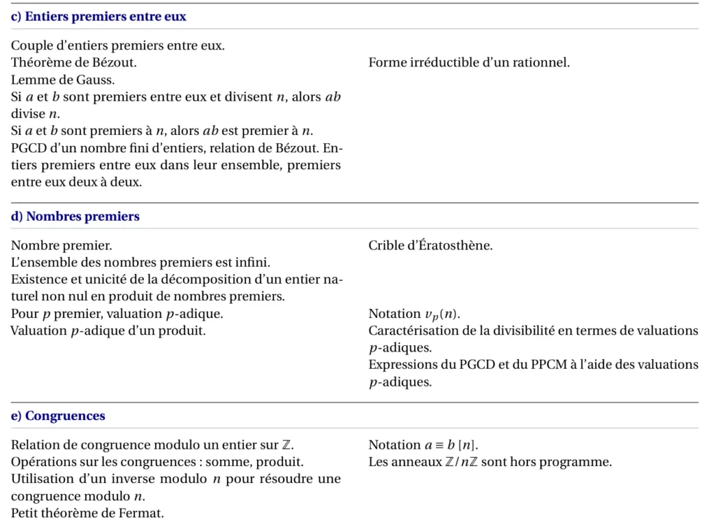
IV) Nombres premiers
Définition 4 : On dit qu’un entier naturel p \geqslant 2 est un nombre premier lorsque D(P)=\{-p,-1,1, p\}. On note \mathbb{P} l’ensemble des nombres premiers.
Remarque 3 : Soit n \in \mathbb{N} \backslash \{0 ; 1\}. On a : n \in \mathbb{P} \Leftrightarrow\left(\forall p, q \in \mathbb{N}^{*},\quad n=p q \Rightarrow p=1 \text{ ou } q=1\right).
Exercice d’application 5 : Soit n \in \mathbb{N}^{*}. Montrer que si 2^{n}-1 est premier alors n est premier.
Corrigé : On suppose que 2^{n}-1 est premier. Soient a, b \in \mathbb{N}^{*}, on suppose que n=a b. 2^{n}-1=\left(2^{a}\right)^{b}-1=\left(2^{a}-1\right) \sum\limits_{k=0}^{b-1}\left(2^{a}\right)^{k}. Puisque 2^{n}-1 est premier, alors 2^{a}-1=1 ou \sum\limits_{k=0}^{b-1}\left(2^{a}\right)^{k}=1. Donc 2^{a}=2 ou \sum\limits_{k=1}^{b-1}\left(2^{a}\right)^{k}=0. Donc a=1 ou b=1. Donc n est premier.
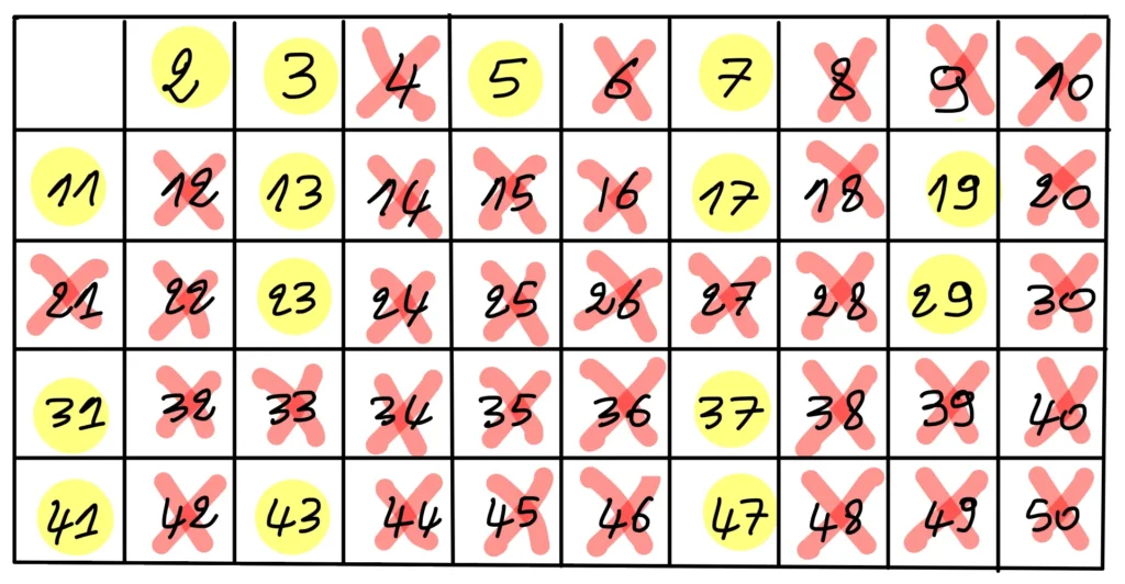
Crible d’Eratosthène : On va donner la liste des nombres premiers inférieurs à 50 en utilisant le crible d’Eratosthène : La méthode est comme suit : \bullet On écrit d’abord tous les entiers compris entre 2 et 50. \bullet Le plus petit de ces nombres est premier, ainsi 2 est premier. \bullet On élimine tous les multiples de 2. \bullet Le plus petit des nombres restant est premier, ainsi 3 est premier. \bullet En réitérant ce procédé, on obtient tous les nombres premiers inférieurs à 50.
Proposition 7 : Soient p un nombre premier et k \in \mathbb{Z}. Si p ne divise pas k, alors p \wedge k=1 En particulier, \forall n \in \llbracket 1, p-1 \rrbracket, n \wedge p=1.
Démonstration : On suppose que p \nmid k. Puisque p \wedge k | p, alors p \wedge k=1 ou p \wedge k=p. Si p \wedge k=p, alors p | k, ce qui est absurde. Donc p \wedge k=1.
Corollaire 1 : Soient n \in \mathbb{N}^{*}, p \in \mathbb{P}, et a_{1}, \cdots, a_{n} \in \mathbb{Z}. p | \prod\limits\limits_{i=1}^{n} a_{i} \Leftrightarrow \exists i \in \llbracket 1, n \rrbracket, p | a_{i}.
Démonstration : « \Leftarrow » Immédiat. "\Rightarrow " On va utiliser la contraposée. On suppose que \forall i \in \llbracket 1, n \rrbracket, \quad \mathrm{p} \nmid a_{i}. Puisque p est premier, \forall i \in \llbracket 1, n \rrbracket, p \wedge a_{i}=1. Donc p \wedge \prod\limits_{i=1}^{n} a_{i}=1. Donc p \nmid \prod\limits_{i=1}^{n} a_{i}. D’où par contraposée p\left|\prod\limits_{\mathrm{i}=1}^{\mathrm{n}} a_{i} \Rightarrow \exists i \in \llbracket 1, n \rrbracket, p\right| a_{i}.
Démonstration : On va d’abord démontrer le résultat par récurrence forte pour n \in \mathbb{N} \setminus \{0 ; 1 \} . \bullet Pour n=2, p=2 convient. \bullet Soit n \in \mathbb{N} \backslash \{0 ; 1 \} . On suppose que \forall k \in \llbracket 2, n \rrbracket, \exists p \in \mathbb{P}, p | k. 1{ \text{er}} cas : Si n+1 est premier. Alors p=n+1 convient. 2{ \text{ème}} cas: Si n+1 n’est pas premier. Alors on peut écrire n+1=a \times b, avec a, b \in \llbracket 2, n \rrbracket . Par hypothèse de récurrence, on sait que \exists p \in \mathbb{P} tels que p |a. Par transitivité, p| n+1. \bullet Par le principe de la récurrence forte, on conclut que pour tout entier n \geq 2, on peut trouver un nombre premier p qui divise p | n .
Maintenant si n \in \mathbb{Z}^{-} \backslash\{-1 ; 0\}, \exists p \in \mathbb{P}, p |-n, et ainsi p | n. D’où \forall n \in \mathbb{Z} \backslash\{-1 ; 0 ; 1\}, \exists p \in \mathbb{P}, p | n.
Démonstration : On suppose que \mathbb{P} est fini. On pose \mathbb{P}=\left\{p_{1} ; \ldots ; p_{n}\right\} et M=p_{1} \times \ldots \times p_{n}+1. On sait que \exists p \in \mathbb{P}, p | M. Comme p | p_{1} \times \ldots \times p_{n}, on trouve p | M-p_{1} \times \ldots \times p_{n}. D’où p | 1. Absurde car p est premier.
Existence : Montrons par récurrence forte que : \forall n \in \mathbb{N} \backslash{0,1}, \exists k \in \mathbb{N}^{*}, \exists\left(p_{1}, \ldots, p_{k}\right) \in \mathbb{P}^{k}, n=\prod\limits_{i=1}^{k} p_{i}. \bullet Pour n=2, on peut écrire n=\prod\limits_{i=1}^{k} p_{i} avec k=1 et p_{1}=2. \bullet Soit n \in \mathbb{N} \backslash\left\{0,1\right\}. On suppose que \forall a \in \llbracket 2, n \rrbracket, \exists k \in \mathbb{N}^{*}, \exists\left(p_{1}, \ldots, p_{k}\right) \in \mathbb{P}^{k}, a=\prod\limits_{i=1}^{k} p_{i}. 1^{e r} cas : Si n+1 est premier. On peut écrire n+1=\prod\limits_{i=1}^{k} p_{i} avec k=1 et p_{1}=n+1. 2^{\text {ème }} cas : Si n+1 n’est pas premier. Dans ce cas \exists a, b \in \llbracket 2, n \rrbracket, n+1=a b. Par hypothèse de récurrence : \exists k_{1} \in \mathbb{N}^{}, \exists\left(p_{1}, \ldots, p_{k_{1}}\right) \in \mathbb{P}^{k_{1}}, a=\prod\limits_{i=1}^{k_{1}} p_{i} et \exists k_{2} \in \mathbb{N}^{}, \exists\left(p_{k_{1}+1}, \ldots, p_{k_{1}+k_{2}}\right) \in \mathbb{P}^{k_{2}}, b=\prod\limits_{i=k_{1}+1}^{k_{1}+k_{2}} p_{i}. Par produit n+1=\prod\limits_{i=1}^{k_{1}+k_{2}} p_{i}. \bullet D’où la partie existence par le principe de la récurrence forte. Unicité : Soit n \in \mathbb{N} \backslash \{0 ; 1\}. On suppose que \exists \mathrm{r}, \mathrm{s} \in \mathbb{N}^{*}, \exists p_{1}, \ldots, p_{r}, q_{1}, \ldots, q_{\mathrm{s}} \in \mathbb{P}, tels que n=p_{1} \times \cdots \times p_{r}=q_{1} \times \cdots \times q_{\mathrm{s}}. On suppose que r<s. On a p_{1} | q_{1} \times \cdots \times q_{\mathrm{s}}, donc \exists \sigma(1) \in \llbracket 1, s \rrbracket, p_{1}=q_{\sigma(1)}. En simplifiant par p_{1}, on trouve : p_{2} \times \cdots \times p_{r}=\prod\limits_{i \in \llbracket 1, s \rrbracket \backslash \{\sigma(1) \} } p_{i}. Quitte à itérer ce procédé, on trouve : 1=\prod\limits_{\substack{i=1 \ i \notin{\sigma(1), \ldots, \sigma(\mathrm{r})}}}^{s} q_{i} \geqslant 2. Donc r \geqslant s. Puisque r et s jouent des rôles symétriques, on obtient également r \leqslant s. Donc \mathrm{r}=s. Et on a \forall i \in \llbracket 1, r \rrbracket, \exists ! \sigma(i) \in \llbracket 1, r \rrbracket, p_{i}=q_{\sigma(i)}. D’où l’unicité de la décomposition de n en produit de nombres premiers.
Remarque 4 : Soit n \in \mathbb{N} \backslash \{0,1\}. \bullet \ \exists ! k \in \mathbb{N}^{}, \exists\left(p_{1}, \ldots, p_{k}\right) \in \mathbb{P} unique à permutation près, \exists !\left(v_{p_{1}}(n), \ldots, v_{p_{k}}(n)\right) \in \mathbb{N}^{}, tels que n=\prod\limits_{i=1}^{k} p_{i}^{v_{P_{i}}(k)}. \bullet Cette écriture est appelée décomposition primaire de n. \bullet \ p_{1}, \ldots, p_{k} sont appelés les facteurs premiers de n. \bullet \ \forall i \in \llbracket 1, k \rrbracket, v_{p_{i}}(n) est appelé valuation p_{i}-adique de n.
Exemple 9 : La décomposition primaire de 90 est : 90=2^{2} \times 3^{2} \times 5^{1}. Ainsi v_{2}(90)=1; v_{3}(90)=2; v_{5}(90)=1.
Remarque 5 : \bullet On généralise ce théorème pour n \in \mathbb{Z} \backslash \{-1 ; 0\} en multipliant la décomposition primaire de -n par -1. \bullet On convient que \forall_{n} \in \mathbb{Z}^{*}, \forall p \in \mathbb{P},\quad v_{p}(n)=0 \Leftrightarrow p \nmid n. \bullet On aura ainsi \forall \mathrm{n} \in \mathbb{Z}^{*}, n=\prod\limits_{p \in \mathbb{P}} p^{v_{p}(n)}.
Exemple 10 : v_{7}(90)=0.
Remarque 6 : \bullet \ \forall p \in \mathbb{P}, v_{p}(p)=1. \bullet \ \forall a, b \in \mathbb{Z}^{*}, \forall p \in \mathbb{P}, v_{p}(a b)=v_{p}(a)+v_{p}(b). \bullet \ \forall n \in \mathbb{N}, \forall a \in \mathbb{Z}^{*}, v_{p}\left(a^{\mathrm{n}}\right)=n v_{p}(a).
Exercice d’application 6 : Montrer que \forall p \in \mathbb{P}, \sqrt{p} \notin \mathbb{Q}.
Corrigé : Soit p \in \mathbb{P}. On suppose par l’absurde que \sqrt{p} \in \mathbb{Q}. Donc \exists a, b \in \mathbb{N}^{*}, \sqrt{p}=\frac{a}{b}. Par suite p b^{2}=a^{2}. D’où v_{p}\left(p b^{2}\right)=v_{p}\left(a^{2}\right). Donc v_{p}(p)+2 v_{p}(b)=2 v_{p}(a). Donc 1+2 v_{p}(b)=2 v_{p}(a). Absurde pour des raisons de parité. Donc \sqrt{p} \notin \mathbb{Q}.
Proposition 9 : Soient a, b \in \mathbb{Z}^{*}, On a : i) a | b \Leftrightarrow \forall p \in \mathbb{P}, v_{p}(a) \leqslant v_{p}(b). ii) a \wedge b=\prod\limits_{p \in \mathbb{P}} p^{\min \left(v_{p}(a), v_{p}(b)\right)}. iii) a \vee b=\prod\limits_{p \in \mathbb{P}} p^{\max \left(v_{p}(a), v_{p}(b)\right)}.
Démonstration : i) " \Rightarrow " On suppose que a | b. Donc \exists c \in \mathbb{Z}, b=a c. Donc \prod\limits_{p \in \mathbb{P}} p^{v_{p}(b)}=b=a c=\prod\limits_{p \in \mathbb{P}} p^{v_{p}(a)+v_{p}(c)}. Par unicité de la valuation-p-adique : \forall p \in \mathbb{P}, v_{p}(b)=v_{p}(a)+v_{p}(c). Comme \forall p \in \mathbb{P}, v_{p}(c) \geq 0, on trouve \forall p \in \mathbb{P}, v_{p}(a) \leqslant v_{p}(b). " \Leftarrow " On suppose que \forall p \in \mathbb{P}, v_{p}(a) \leqslant v_{p}(b). On pose c=\prod\limits_{p \in \mathbb{P}} p^{v_{p}(b)-v_{p}(a)}. Il est évident que a c=b. Donc a | b. ii) On pose d=\prod\limits_{p \in \mathbb{P}} p^{\min \left(v_{p}(a), v_{p}(b)\right)}. Par unicité de la valuation p-adique, \forall p \in \mathbb{P}, v_{p}(d)=\min \left(v_{p}(a), v_{p}(b)\right). On sait que a \wedge b | a et a \wedge b | b. Alors, d’après i), \forall p \in \mathbb{P}, v_{p}(a \wedge b) \leqslant v_{p}(a) et v_{p}(a \wedge b) \leqslant v_{p}(b). Donc \forall p \in \mathbb{P}, v_{p}(a \wedge b) \leqslant \min \left(v_{p}(a), v_{p}(b)\right)=v_{p}(d). Toujours d’après i), on trouve que a \wedge b | d. Il est clair que \forall p \in \mathbb{P}, v_{p}(d) \leqslant v_{p}(a) et v_{p}(d) \leqslant v_{p}(b). Donc en appliquant i), d | a et d | b. Donc d | a \wedge b. Par (*) et (* *) on trouve |d|=|a \wedge b| et par la suite d=a \wedge b.
Exemple 11 : Calculons 9000 \wedge 1600 et 9000 \vee 1600. La décomposition primaire de 1600 est : 2^{6} \times 5^{2}. La décomposition primaire de 9000 est : 2^{3} \times 3^{2} \times 5^{3}. Donc PGCD(1600,9000)=2^{3} \times 5^{2} et PPCM(1600,9000)=2^{6} \times 3^{2} \times 5^{3}.
V) Congruences
Définition 5 : Soient n \in \mathbb{N} et (a, b) \in \mathbb{Z}. On dit que a est congru à b modulo n et on note a \equiv b[n] lorsque n | a-b.
Remarque 7 : \forall n \in \mathbb{N}, \forall a, b \in \mathbb{Z}, \quad a \equiv b[n] \Leftrightarrow \exists k \in \mathbb{Z}, a=b+n k.
Compatibilité de la congruence avec les opérations : Soient n \in \mathbb{N} et a, b, c, d \in \mathbb{Z}. Si a \equiv b[n] et c \equiv d[n] alors : i) a+c \equiv b+d[n]. ii) a c \equiv b d[n]. iii) \forall k \in \mathbb{N}, a^{k} \equiv b^{k}[n]. iv) La relation de congruence modulo un entier n \in \mathbb{N} est une relation d’équivalence sur \mathbb{Z}.
Démonstration : On suppose que \equiv \mathrm{b}[n] et c \equiv \mathrm{d}[n]. i) On a a \equiv b[n] donc n | a-b. Et on a c \equiv d[n] donc n | c-d. Donc n | a-b+c-d ou encore n |(a+c)-(b+d). Ce qui signifie que a+c \equiv b+d[n]. ii) On a a \equiv b[n] donc \exists k \in \mathbb{Z}, a=b+k n. Et on a c \equiv d[n] donc \exists k^{\prime} \in \mathbb{Z}, c=d+k^{\prime} n Par produit a c=b d+n\left(b k^{\prime}+d k+n b k^{\prime}\right). Finalement a c \equiv b d[n]. iii) Une simple récurrence utilisant ii). iv) On vérifie facilement que la relation est réflexive, symétrique et transitive.
Petit théorème de Fermat : i) \forall p \in \mathbb{P}, \forall n \in \mathbb{Z}, n^{p} \equiv n[p]. ii) \forall p \in \mathbb{P}, \forall n \in \mathbb{Z}, \quad n \wedge p=1 \Rightarrow n^{p-1} \equiv 1[p].
i) Soit p \in \mathbb{P}. Montrons d’abord par récurrence que \forall n \in \mathbb{N}, n^{p} \equiv n[p] \bullet \text{ Pour } n=0 \text{ on a } 0^{p} \equiv 0[p]. \bullet Soit n \in \mathbb{N}. On suppose que n^{p} \equiv n[p]. (n+1)^{p}=\sum\limits_{k=0}^{p}\binom{p}{k} n^{k}=1+n^{p}+\sum\limits_{k=1}^{p-1} \binom{p}{k} n^{k}. Or \forall k \in \llbracket 1, p-1 \rrbracket, p \wedge k=1 car p est premier. Donc d’après l’exercice d’application 4 trouve que \forall k \in \llbracket 1, p-1 \rrbracket, \ \binom{p}{k} \equiv 0[p]. Et par la suite (n+1)^{p} \equiv 1+n^{p}[p] \equiv n+1[p]. \bullet On conclut par le principe de la récurrence que \forall n \in \mathbb{N}, n^{p} \equiv n[p].
Généralisons ce résultat à \mathbb{Z}. Soit n \in \mathbb{Z}^{-}. 1^{e r} cas : Si p=2 p est pair donc (-n)^{p}=n^{p}. Puisque -n \in \mathbb{N} par ce qui précède on trouve (-n)^{p} \equiv-n[p]. Donc n^{p} \equiv-n[p]. Puisque -n \equiv n[p] alors n^{p} \equiv n[p]. 2^{\text {ème }} cas : \operatorname{si} p \geqslant 3. Puisque p est impair alors (-n)^{p}=-n^{p}. Puisque -n \in \mathbb{N} par ce qui précède on trouve (-n)^{p} \equiv-n[p]. Donc -n^{p} \equiv-n[p] ou encore n^{p} \equiv n[p].
Conclusion : \forall p \in \mathbb{P}, \forall n \in \mathbb{Z}, n^{p} \equiv n[p].
ii) Soit p \in \mathbb{P} et n \in \mathbb{Z} tels que n \wedge p=1. Par i) on a n^{p} \equiv n[p]. Ce qui se traduit par p | n^{p}-n ou encore p | n\left(n^{p-1}-1\right). Comme n \wedge p=1 par le théorème de Gauss p | n^{p-1}-1. Autrement dit n^{p-1} \equiv 1[p].