Ce cours sur le calcul matriciel et systèmes linéaires est conforme au programme des filières MPSI et MP2I. Il contient des exemples et des exercices d’application qui faciliteront votre assimilation du contenu. N’hésitez pas à consulter notre série d’exercices corrigés pour acquérir une maîtrise solide de cours.
Le but de ce chapitre est de présenter une initiation au calcul matriciel. Ainsi, on prépare l’étude géométrique de l’algèbre
linéaire menée au second semestre, on revient sur l’étude des systèmes linéaires et on obtient des exemples fondamentaux
d’anneaux.
Dans tout ce chapitre et sauf mention explicite du contraire, n, p et q sont trois entiers naturels non nuls et \mathbb{K} désigne \mathbb{R} ou \mathbb{C}.
I) Opérations sur les matrices
Définition 1 :
On appelle matrice à n lignes et p colonnes à coefficients dans \mathbb{K}, toute famille \left(a_{i j}\right)_{\substack{i \in \llbracket 1, n \rrbracket \\ j \in \llbracket 1, p \rrbracket}} d’éléments de \mathbb{K}.
On note \left(a_{i j}\right)_{\substack{i \in \llbracket 1, n \rrbracket \\ j \in \llbracket 1, p \rrbracket}}=\left(a_{i j}\right)_{\substack{1 \leq i \leq n \\ 1 \leq j \leq p}}=\left(\begin{array}{ccc}a_{1,1} & \ldots & a_{1, p} \\ \vdots & \ddots & \vdots \\ a_{n, 1} & \ldots & a_{n, p}\end{array}\right)=A.
\bullet Les a_{i j} sont appelés coefficients de la matrice A.
\bullet (n, p) est appelé taille ou format de la matrice.
\bullet On note \mathcal{M}_{n, p}(\mathbb{K}) l’ensemble des matrices à n lignes et p colonnes à coefficients dans \mathbb{K}.
\bullet Lorsque n=p, on dit que A est une matrice carrée et on note \mathcal{M}_{n, p}(\mathbb{K})=\mathcal{M}_{n}(\mathbb{K}).
Remarque 1 :
Soient A=\left(a_{i j}\right) et B=\left(b_{i j}\right) deux matrices de \mathcal{M}_{n, p}(\mathbb{K}).
A=B \Leftrightarrow \forall(i, j) \in \llbracket 1, n \rrbracket \times \llbracket 1, p \rrbracket, \ a_{i j}=b_{i j}.
Exemple 1 :
i) On pose A=\begin{pmatrix}1 & -1 & 0 \\ \sqrt{2} & \frac{3}{2} & \pi\end{pmatrix}=\left(a_{i j}\right)_{\substack{1 \leq i \leq 2 \\ 1 \leq j \leq 3}} \in \mathcal{M}_{2,3}(\mathbb{K}). On a alors :
a_{1,1}=1 ; a_{1,2}=-1 ; a_{1,3}=0 ; a_{2,1}=\sqrt{2} ; a_{2,2}=\frac{3}{2} ; a_{2,3}=\pi.
ii) A=\begin{pmatrix} 1 \\ i \\ \sqrt{2}\end{pmatrix} \in \mathcal{M}_{3,1}(\mathbb{C}) est une matrice colonne.
iii) A=\begin{pmatrix}-1 & \sqrt{2} & i & \frac{5}{3}\end{pmatrix} \in \mathcal{M}_{1,4}(\mathbb{C}) est une matrice ligne.
iv) On appelle matrice identité de \mathcal{M}_{n}(\mathbb{K}), et on note I_{n}, la matrice à n lignes et n colonnes dont tous les coefficients sont nuls sauf ceux de la diagonale qui sont égaux à 1.
Pour tout i, j \in \llbracket 1, n \rrbracket, on définit le réel \delta_{i, j} qu’on appelle symbole de Kronecker, par : \delta_{i, j}=\begin{cases}1, \text { si } i=j \\ 0, \text { si } i \neq j\end{cases}.
On écrit alors I_{n}=\left(\delta_{i, j}\right)_{1 \leq i, j \leq n}.
Par exemple, dans \mathcal{M}_{3}(\mathbb{K}), I_{3}=\begin{pmatrix}1 & 0 & 0 \\ 0 & 1 & 0 \\ 0 & 0 & 1\end{pmatrix} et dans \mathcal{M}_{2}(\mathbb{K}), I_{2}=\begin{pmatrix}1 & 0 \\ 0 & 1\end{pmatrix}.
v) On appelle matrice nulle de \mathcal{M}_{n, p}(\mathbb{K}), et on note 0_{\mathcal{M}_{n, p}(\mathbb{K})} ou 0_{n, p} ou tout simplement 0, la matrice à n lignes et p colonnes dont tous les coefficients sont nuls.
Par exemple, dans \mathcal{M}_{3,2}(\mathbb{K}), 0=\begin{pmatrix}0 & 0 \\ 0 & 0 \\ 0 & 0\end{pmatrix} et dans \mathcal{M}_{2,3}(\mathbb{R}), 0=\begin{pmatrix}0 & 0 & 0 \\ 0 & 0 & 0\end{pmatrix}.
Addition, multiplication par un scalaire :
Soient A, B \in \mathcal{M}_{n, p}(\mathbb{K}) et \lambda, \mu \in \mathbb{K}. On pose A=\left(a_{i j}\right)_{\substack{i \in \llbracket 1, n \rrbracket \\ j \in \llbracket 1, p \rrbracket}} et B=\left(b_{i j}\right)_{\substack{i \in \llbracket 1, n \rrbracket \\ j \in \llbracket 1, p \rrbracket}}.
i) On appelle somme de A et B, et on note A+B, la matrice de \mathcal{M}_{n, p}(\mathbb{K}) définie par A+B=\left(a_{i j}+b_{i j}\right)_{ \substack{1 \leqslant i \leqslant n \\ 1 \leqslant j \leqslant p}}.
ii) On appelle produit de la matrice A par le scalaire \lambda, et on note \lambda A, la matrice de \mathcal{M}_{n, p}(\mathbb{K}) définie par : \lambda A=\left(\lambda a_{i j}\right)_{\substack{1 \leqslant i \leqslant n \\ 1 \leqslant j \leqslant p}}.
Exemple 2 :
i) \begin{pmatrix}1 & 0 \\ -1 & 1\end{pmatrix}+\begin{pmatrix}-1 & \pi \\ 0 & 1\end{pmatrix}=\begin{pmatrix}0 & \pi \\ -1 & 2\end{pmatrix}.
ii) L’opération \begin{pmatrix}0 & 0 \\ -1 & 1 \\ 1 & 1\end{pmatrix}+\begin{pmatrix}1 & 1 & 1 \\ -1 & 0 & 1 \\ 0 & 1 & 0\end{pmatrix} n’est pas définie.
iii) 2 \cdot\begin{pmatrix}1 & -1 \\ 0 & 2 \\ \sqrt{2} & \pi\end{pmatrix}=\begin{pmatrix}2 & -2 \\ 0 & 4 \\ 2 \sqrt{2} & 2 \pi\end{pmatrix}.
Combinaison linéaire de matrices :
Soient k \in \mathbb{N}^{*}, A_{1}, \ldots, A_{k} k matrices de \mathcal{M}_{n, p}(\mathbb{K}) telles que \forall q \in \llbracket 1, k \rrbracket, A_{q}=\left(a_{i j}(q)\right)_{ \substack{1 \leqslant i \leqslant n \\ 1 \leqslant j \leqslant p}} et \lambda_{1}, \ldots, \lambda_{k} k-scalaires.
\sum\limits_{i=1}^{k} \lambda_{i} A_{i} est dite combinaison linéaire des matrices A_{1}, \ldots, A_{k}.
Et on a: \sum\limits_{i=1}^{k} \lambda_{i} A_{i}=\left(\sum\limits_{q=1}^{k} \lambda_{q} a_{i, j}(q)\right)_{\substack{1 \leq i \leq n \\ 1 \leqslant j \leqslant p}}.
Matrices élémentaires :
Soit (i, j) \in \llbracket 1, n \rrbracket \times \llbracket 1, p \rrbracket.
Dans \mathcal{M}_{n, p}(\mathbb{K}), on note E_{i j} la matrice à n lignes et p colonnes, dont tous les coefficients sont nuls sauf celui situé à l’intersection de la i^{\text {ème }} ligne et la j ème colonne qui vaut 1.
On peut écrire dans ce cas E_{i j}=\left(e_{r, s}\right)_{1 \leqslant r \leqslant n, 1 \leqslant s \leqslant p} où \forall(r, s) \in \llbracket 1, n \rrbracket \times \llbracket 1, p \rrbracket, e_{r, s}=\delta_{r i} \delta_{s, j} . E_{i, j} est dite matrice élémentaire.
Exemple 3 :
\bullet Dans \mathcal{M}_{3}(\mathbb{R}), \ E_{1,2}=\begin{pmatrix}0 & 1 & 0 \\ 0 & 0 & 0 \\ 0 & 0 & 0\end{pmatrix}.
\bullet Dans \mathcal{M}_{3,2}(\mathbb{R}), \ E_{12}=\begin{pmatrix}0 & 1 \\ 0 & 0 \\ 0 & 0\end{pmatrix}.
\bullet Dans \mathcal{M}_{2,3}(\mathbb{R}), \ E_{12}=\begin{pmatrix}0 & 1 & 0 \\ 0 & 0 & 0\end{pmatrix}.
Proposition 1 :
Toute matrice de \mathcal{M}_{n, p}(\mathbb{K}) est combinaison linéaire de matrices élémentaires.
Plus précisément si A est une matrice de \mathcal{M}_{n, p}(\mathbb{K}) et \left(a_{i j}\right)_{\substack{1 \leq i \leq n, 1 \leqslant j \leqslant p}} est une famille de scalaires de \mathbb{K}, alors :
A=\left(a_{i j}\right)_{\substack{1 \leq i \leq n, 1 \leqslant j \leqslant p}} \Leftrightarrow A=\sum\limits_{i=1}^{n} \sum\limits_{j=1}^{p} a_{i j} E_{i j}.
Produit matriciel :
Soient A \in \mathcal{M}_{n, p}(\mathbb{K}) et B \in \mathcal{M}_{p, q}(\mathbb{K}). On pose A=\left(a_{i j}\right)_{\substack{1 \leq i \leq n \\ 1 \leqslant j \leqslant p}} et B=\left(b_{i j}\right)_{\substack{1 \leq i \leq p \\ 1 \leqslant j \leqslant q}}.
Le produit des deux matrices A et B, qu’on note A B, est une matrice de \mathcal{M}_{n, q}(\mathbb{K}), définie par A B=\left(c_{i j}\right)_{\substack{1 \leq i \leq n \\ 1 \leqslant j \leqslant q}} avec \forall(i, j) \in \llbracket 1, n \rrbracket \times \llbracket 1, q \rrbracket, c_{i, j}=\sum\limits_{k=1}^{p} a_{i k} b_{k j}.
Exemple 4 :
i) \begin{pmatrix}0 & -1 \\ 1 & 2 \\ 0 & 1\end{pmatrix} \begin{pmatrix}1 & -1 & 0 & 2 \\ 0 & 1 & 3 & 0\end{pmatrix}=\begin{pmatrix}0 & -1 & -3 & 0 \\ 1 & 1 & 6 & 2 \\ 0 & 1 & 3 & 0\end{pmatrix}.
ii) L’opération \begin{pmatrix}1 & -1 & 0 & 2 \\ 0 & 1 & 3 & 0\end{pmatrix}\begin{pmatrix}0 & -1 \\ 1 & 2 \\ 0 & 1\end{pmatrix} n’est pas définie.
iii) \begin{pmatrix}1 \\ 0 \\ -1\end{pmatrix}\begin{pmatrix}2 & 0 & 1\end{pmatrix}=\begin{pmatrix}2 & 0 & 1 \\ 0 & 0 & 0 \\ -2 & 0 & -1\end{pmatrix} et \begin{pmatrix}2 & 0 & 1\end{pmatrix}\begin{pmatrix}1 \\ 0 \\ -1\end{pmatrix}=1.
iv) \begin{pmatrix}1 & 0 \\ -1 & 2\end{pmatrix}\begin{pmatrix}-1 & 1 \\ 0 & -2\end{pmatrix}=\begin{pmatrix}-1 & 1 \\ 1 & -5\end{pmatrix} et \begin{pmatrix}-1 & 1 \\ 0 & -2\end{pmatrix}\begin{pmatrix}1 & 0 \\ -1 & 2\end{pmatrix}=\begin{pmatrix}-2 & 2 \\ 2 & -4\end{pmatrix}.
En particulier on remarque que \begin{pmatrix}1 & 0 \\ -1 & 2\end{pmatrix}\begin{pmatrix}-1 & 1 \\ 0 & -2\end{pmatrix} \neq\begin{pmatrix}-1 & 1 \\ 0 & -2\end{pmatrix}\begin{pmatrix}1 & 0 \\ -1 & 2\end{pmatrix}
Ce qui signifie que le produit matriciel n’est pas commutatif dans le cas général.
v) \begin{pmatrix}0 & 1 \\ 0 & 0\end{pmatrix}\begin{pmatrix}0 & 1 \\ 0 & 0\end{pmatrix}=\begin{pmatrix}0 & 0 \\ 0 & 0\end{pmatrix}=0.
Ainsi A B=0 \nRightarrow A=0 ou B=0.
Ou encore A \neq 0 et B \neq 0 \nRightarrow A B \neq 0.
Remarque 2 :
Pour toute matrice A de \mathcal{M}_{n, p}(\mathbb{K}) on a :
\bullet A I_{p}=A .
\bullet I_{n} A=A .
\bullet 0_{\mathcal{M}_{q, n}(\mathbb{K})} \times A=0_{\mathcal{M}_{q, p}(\mathbb{K})} .
\bullet A \times 0_{\mathcal{M}_{p, q}(\mathbb{K})}=0_{\mathcal{M}_{n, q}(\mathbb{K})}.
Exemple 5 :
\bullet \begin{pmatrix}1 & 0 & 0 \\ 0 & 0 & 0\end{pmatrix}\begin{pmatrix}0 & 0 \\ 1 & 0 \\ 0 & 0\end{pmatrix}=E_{1,1}\left(\mathcal{M}_{2,3}(\mathbb{R})\right) \times E_{21}\left(\mathcal{M}_{3,2}(\mathbb{R})\right)=0.
\bullet \begin{pmatrix}0 & 1 \\ 0 & 0\end{pmatrix}\begin{pmatrix}0 & 0 \\ 0 & 1\end{pmatrix}=E_{12} E_{22}=\delta_{2,2} E_{12}=E_{12}=\begin{pmatrix}0 & 1 \\ 0 & 0\end{pmatrix}.
Produit d’une matrice par une matrice colonne :
Soient A=\left(a_{i j}\right)_{\substack{1 \leq i \leq n \\ 1 \leqslant j \leqslant p}} une matrice de \mathcal{M}_{n, p}(\mathbb{K}) et X=\begin{pmatrix}x_{1} \\ \vdots \\ x_{p}\end{pmatrix} une matrice colonne de \mathcal{M}_{p, 1}(\mathbb{K}).
Pour tout i \in \llbracket 1, p \rrbracket, on note C_{i}(A) la i^{\text {ème }} colonne de A.
Alors on a A X=\begin{pmatrix}\sum\limits_{j=1}^{p} a_{1 j} x_{j} \\ \vdots \\ \sum\limits_{j=1}^{p} a_{n j} x_{j}\end{pmatrix}=\sum\limits_{j=1}^{p} x_{j} C_{j}(A).
Transposée d’une matrice :
Soit A=\left(a_{i, j}\right) une matrice de \mathcal{M}_{n, p}(\mathbb{K}).
On appelle transposée de A et on note A^{\top} (ou \left.t_{A}\right), la matrice \left(b_{i j}\right) de \mathcal{M}_{p, n}(\mathbb{K}) définie par : \forall(i, j) \in \llbracket 1, p \rrbracket \times \llbracket 1, n \rrbracket,\ b_{i j}=a_{j, i}.
Exemple 6 :
i) \begin{pmatrix}1 & 0 & -1 \\ \sqrt{2} & \pi & 0\end{pmatrix}^{\top}=\begin{pmatrix}1 & \sqrt{2} \\ 0 & \pi \\ -1 & 0\end{pmatrix}.
ii) \begin{pmatrix}1 & -1 \\ 2 & 3\end{pmatrix}^{\top}=\begin{pmatrix}1 & 2 \\ -1 & 3\end{pmatrix}.
iii) \begin{pmatrix}1 & -1 & 0\end{pmatrix}^{\top}=\begin{pmatrix}1 \\ -1 \\ 0\end{pmatrix}.
II) Opérations élémentaires
Définition 2 :
Soient i, j \in \llbracket 1, n \rrbracket tels que i \neq j et \lambda \in \mathbb{K}^{*}.
i) On pose T_{i j}(\lambda)=I_{n}+\lambda E_{i j}, une matrice de cette forme est dite matrice de transvection. (La matrice T_{i j}(\lambda) est obtenue en appliquant l’opération L_{i} \leftarrow L_{i}+\lambda L_{j} à la matrice I_{n}).
ii) On pose P_{i j}=I_{n}-E_{i i}-E_{j j}+E_{i j}+E_{j i}, une matrice de cette forme est dite matrice transposition. (La matrice P_{i j} est obtenue en appliquant l’opération L_{i} \leftrightarrow L_{j} à la matrice I_{n}).
iii) On pose D_{i}(\lambda)=I_{n}+(\lambda-1) E_{i i}, une matrice de cette forme est dite matrice de dilation. (La matrice D_{i}(\lambda) est obtenue en appliquant l’opération L_{i} \leftarrow \lambda L_{i} à la matrice I_{n}).
Exemple 7 :
Soient A=\left(a_{i j}\right) une matrice de \mathcal{M}_{3}(\mathbb{R}) et \lambda un nombre réel.
Dans \mathcal{M}_{3}(\mathbb{R}), effectuer les opérations suivantes :
\bullet \ T_{2,3}(\lambda) A=\begin{pmatrix}1 & 0 & 0 \\ 0 & 1 & \lambda \\ 0 & 0 & 1\end{pmatrix}\begin{pmatrix}a_{1,1} & a_{1,2} & a_{1,3} \\ a_{2,1} & a_{2,2} & a_{2,3} \\ a_{3,1} & a_{3,2} & a_{3,3}\end{pmatrix}=\begin{pmatrix}a_{1,1} & a_{2,2} & a_{1,3} \\ a_{2,1}+\lambda a_{3,1} & a_{2,2}+\lambda a_{3,2} & a_{2,3}+\lambda a_{3,3} \\ a_{3,1} & a_{3,2} & a_{3,3}\end{pmatrix}.
\bullet \ P_{2,1} A=\begin{pmatrix}0 & 1 & 0 \\ 1 & 0 & 0 \\ 0 & 0 & 1\end{pmatrix}\begin{pmatrix}a_{1,1} & a_{1,2} & a_{1,3} \\ a_{2,1} & a_{2,2} & a_{2,3} \\ a_{3,1} & a_{3,2} & a_{3,3}\end{pmatrix}=\begin{pmatrix}a_{2,1} & a_{2,2} & a_{2,3} \\ a_{1,1} & a_{1,2} & a_{1,3} \\ a_{3,1} & a_{3,2} & a_{3,3}\end{pmatrix}.
\bullet \ D_{2}(\lambda) A=\begin{pmatrix}1 & 0 & 0 \\ 0 & \lambda & 0 \\ 0 & 0 & 2\end{pmatrix}\begin{pmatrix}a_{1,1} & a_{1,2} & a_{1,3} \\ a_{2,1} & a_{2,2} & a_{2,3} \\ a_{3,1} & a_{3,2} & a_{3,3}\end{pmatrix}=\begin{pmatrix}a_{1,1} & a_{1,2} & a_{1,3} \\ \lambda a_{2,1} & \lambda a_{2,2} & \lambda a_{2,3} \\ a_{3,1} & a_{3,2} & a_{3,3}\end{pmatrix}.
\bullet \ A T_{2,1}(\lambda)=\begin{pmatrix}a_{1,1} & a_{1,2} & a_{1,3} \\ a_{2,1} & a_{2,2} & a_{2,3} \\ a_{3,1} & a_{3,2} & a_{3,3}\end{pmatrix}\begin{pmatrix}1 & 0 & 0 \\ \lambda & 1 & 0 \\ 0 & 0 & 1\end{pmatrix}=\begin{pmatrix}a_{1,1}+\lambda a_{1,2} & a_{1,2} & a_{1,3} \\ a_{2,1}+\lambda a_{2,2} & a_{2,2} & a_{2,3} \\ a_{3,1}+\lambda a_{3,2} & a_{3,2} & a_{3,3}\end{pmatrix}.
\bullet \ A P_{2,3}=\begin{pmatrix}a_{1,1} & a_{1,2} & a_{1,3} \\ a_{2,1} & a_{2,2} & a_{2,3} \\ a_{3,1} & a_{3,2} & a_{3,3}\end{pmatrix}\begin{pmatrix}1 & 0 & 0 \\ 0 & 0 & 1 \\ 0 & 1 & 0\end{pmatrix}=\begin{pmatrix}a_{1,1} & a_{1,3} & a_{1,2} \\ a_{2,1} & a_{2,3} & a_{2,2} \\ a_{3,1} & a_{3,3} & a_{3,2}\end{pmatrix}.
\bullet \ A D_{1}(\lambda)=\begin{pmatrix}a_{1,1} & a_{1,2} & a_{1,3} \\ a_{2,1} & a_{2,2} & a_{2,3} \\ a_{3,1} & a_{3,2} & a_{3,3}\end{pmatrix}\begin{pmatrix}\lambda & 0 & 0 \\ 0 & 1 & 0 \\ 0 & 0 & 1\end{pmatrix}=\begin{pmatrix}\lambda a_{1,1} & a_{1,2} & a_{1,3} \\ \lambda a_{2,1} & a_{2,2} & a_{2,3} \\ \lambda a_{3,1} & a_{3,2} & a_{3,3}\end{pmatrix}.
Interprétation des opérations élémentaires sur les lignes et sur les colonnes en termes de produit matriciel :
i) Opérations sur les lignes :
Soient A \in M_{n, p}(\mathbb{K}), \lambda \in \mathbb{K}^{*} et i, j deux entiers distincts de \llbracket 1, n \rrbracket.
\bullet Le produit matriciel T_{i j}(\lambda) A revient à appliquer l’opération élémentaire L_{i} \leftarrow L_{i}+\lambda L_{j} sur la matrice A.
\bullet Le produit matriciel P_{i j} A revient à appliquer l’opération élémentaire L_{i} \leftrightarrow L_{j} sur la matrice A.
\bullet Le produit matriciel D_{i}(\lambda) A revient à appliquer l’opération élémentaire L_{i} \leftarrow \lambda L_{i} sur la matrice A.
ii) Opérations sur les colonnes :
Soient A \in M_{n, p}(\mathbb{K}), \lambda \in \mathbb{K}^{*} et i, j deux entiers distincts de \llbracket 1, p \rrbracket.
\bullet Le produit matriciel A T_{i j}(\lambda) revient à appliquer l’opération élémentaire C_{j} \leftarrow C_{j}+\lambda C_{i} sur la matrice A.
\bullet Le produit matriciel A P_{i j} revient à appliquer l’opération élémentaire C_{i} \leftrightarrow C_{j} sur la matrice A.
\bullet Le produit matriciel A D_{i}(\lambda) revient à appliquer l’opération élémentaire C_{i} \leftarrow \lambda C_{i} sur la matrice A.
III) Système linéaire
Soient A=\left(a_{i j}\right) une matrice de \mathcal{M}_{n, p}(\mathbb{K}) et B=\begin{pmatrix}b_{1} \\ \mathrm{~b}_{2} \\ \vdots \\ b_{n}\end{pmatrix} un vecteur colonne de \mathcal{M}_{n, 1}(\mathbb{K}) et on considère le système linéaire (S) de n équations à p inconnues suivant :
(S):\begin{cases}a_{1,1} x_{1}+&a_{1,2} x_{2}+&\cdots+&a_{1, p} x_{p}&=b_{1} \\ \cdots& \cdots& \cdots& \cdots& =\cdots \\ a_{n, 1} x_{1}+&a_{n, 2} x_{2}+&\cdots+&a_{n, p} x_{p}&=b_{p}\end{cases}
\bullet Les a_{i j} sont appelés les coefficients du système (S).
\bullet La matrice A est dite matrice des coefficients du système (S).
\bullet Les b_{i} forment ce que l’on appelle le second membre du système.
\bullet Lorsque les b_{i} sont tous nuls, on dit que le système (\mathrm{S}) est homogène.
\bullet Dans le cas général, on appelle système homogène associé à (S), et on note \left(S_{0}\right), le système de même coefficients que (S) et avec second membre nul.
\bullet On appelle solution du système (S) tout p-uplet \left(x_{1}, \ldots, x_{p}\right) de \mathbb{K}^{p} tel que les n équations de (S) soient vérifiées.
\bullet Un système qui n’admet aucune solution est dit incompatible.
\bullet Un système admettant au moins une solution est dit compatible.
\bullet Tout système homogène est compatible et l’ensemble de ses solutions est stable par combinaisons linéaires.
\bullet Résoudre le système (S) revient à résoudre l’équation A X=B d’inconnue X \in M_{p, 1}(K).
\bullet L’équation A X=B est dite écriture matricielle du système linéaire (S).
\bullet Le système A X=B est compatible si et seulement si B est combinaison linéaire des colonnes de A.
\bullet L’ensemble des solutions d’un système compatible A X=B est X_{0}+S_{0}, où X_{0} est une solution particulière et S_{0} désigne l’ensemble des solutions du système homogène associé A X=0. Avec la notation X_{0}+S_{0}=\left\{X_{0}+Y / Y \in S_{0}\right\}.
\bullet Le système linéaire (S) est dit échelonné quand les deux propriétés i) et ii) suivantes sont vérifiées :
i) Si une ligne de A, la matrice des coefficients de (S), est nulle les lignes suivantes le sont aussi.
ii) Quand deux lignes successives de A sont non nulles, l’indice de la colonne du premier coefficient non nul de la ligne supérieure est strictement inférieur à l’indice de la colonne du premier coefficient non nul de la ligne inférieure.
\bullet Chaque premier coefficient non nul d’une ligne d’un système échelonné est appelé pivot.
\bullet Une opération élémentaire sur les lignes (les transvections, les permutations et les dilatations) d’un système linéaire le transforme en un autre système linéaire qui possède le le même ensemble de solutions.
Algorithme du pivot de Gauss :
En utilisant des opérations élémentaires sur les lignes, on peut transformer un système linéaire en un système linéaire échelonné, donc plus facile à résoudre.
IV) Anneau des matrices carrées
Proposition 3 :
\left( \mathbb{M}_{n}(\mathbb{K}),+, \times\right) est un anneau.
Remarque 3 :
i) La matrice nulle, est l’élément neutre pour l’addition dans \left(\mathcal{M}_{n}(\mathbb{k}),+, \times\right).
ii) I_{n}, la matrice identité, est l’élément neutre pour la multiplication dans \left(\mathcal{M}_{n}(\mathbb{K}),+, \times\right).
iii) \left(\mathcal{M}_{n}(\mathbb{K}),+, \times\right) est non commutatif si n \geqslant 2.
En effet E_{1,2} E_{2,1}=E_{1,1} et E_{2,1} E_{1,2}=E_{2,2} donc E_{1,2} E_{2,1} \neq E_{2,1} E_{1,2}.
Définition 3 :
On dit qu’un élément A de \left(\mathbb{M}_{n}(\mathbb{K}),+, \times\right) est nilpotent lorsqu’ il existe un entier naturel p tel que A^{p}=0.
Dans ce cas, le plus petit entier naturel k tel que A^{k}=0 est appelé indice de nilpotence de A.
Par exemple, dans M_{n}(\mathbb{K}), la matrice E_{1,2} est nilpotente car \left(E_{1,2}\right)^{2}=0. Son indice de nilpotence vaut 2.
En particulier la matrice E_{1,2} est un diviseur de zéro dans l’anneau \left(\mathcal{M}_{n}(\mathbb{K}),+, \times\right).
Définition 4 (Matrice symétrique, matrice antisymétrique) :
i) On dit qu’une matrice A de \mathcal{M}_{n}(\mathbb{K}) est symétrique lorsque A^{\top}=A.
On note S_{n}(\mathbb{K}) l’ensemble des matrices symétriques de \mathcal{M}_{n}(\mathbb{K}).
ii) On dit qu’une matrice A de \mathcal{M}_{n}(\mathbb{K}) est antisymétrique lorsque A^{\top}=-A.
On note A_{n}(\mathbb{K}) l’ensemble des matrices antisymétriques de \mathcal{M}_{n}(\mathbb{K}).
Exemples de matrices symétriques et antisymétriques.
i) \begin{pmatrix}0 & -1 \\ -1 & 1\end{pmatrix} est une matrice symétrique
ii) \begin{pmatrix}0 & -1 & -2 \\ 1 & 0 & 3 \\ 2 & -3 & 0\end{pmatrix} est une matrice antisymétrique.
Formule du binôme pour les matrices :
Soient A et B deux matrices de \mathcal{M}_{n}(\mathbb{K}).
Si A et B commutent alors \forall p \in \mathbb{N},(A+B)^{p}=\sum\limits\limits_{k=0}^{p}\binom{p}{k} A^{k} B^{p-k}.
Définition 5 (Matrice diagonale, matrice triangulaire) :
Soit A=\left(a_{i, i}\right){1 \leqslant i, j \leqslant m} une matrice de \mathcal{M}{n}(\mathbb{K}).
i) On dit que A est diagonale lorsque : \forall i, j \in \mathbb{1} 1, m]], i \neq j \Rightarrow a_{i j}=0.
C’est-à-dire A=\begin{pmatrix}a_{1,1} & 0 & \cdots & \cdots & 0 \\ 0 & \ddots & & & \vdots \\ \vdots & \ddots & \ddots & & \vdots \\ \vdots & \ddots & \ddots & & 0 \\ 0 & \cdots & \cdots & 0 & a_{n, n}\end{pmatrix}.
On note dans ce cas A=\operatorname{diag}\left(a_{1,1}, \ldots, a_{n, n}\right).
ii) On dit que A est triangulaire supérieure lorsque : \forall i, j \in \llbracket 1, n \rrbracket, \quad i>j \Rightarrow a_{i, j}=0.
C’est-à-dire A=\begin{pmatrix}a_{1,1} & a_{1,2} & \cdots & \cdots & a_{1, \mathrm{n}} \\ 0 & \ddots & & & \vdots \\ \vdots & \ddots & \ddots & & \vdots \\ \vdots & \ddots & \ddots & & a_{n-1, \mathrm{n}} \\ 0 & \cdots & \cdots & 0 & a_{n, n}\end{pmatrix}.
iii) On dit que A est triangulaire inférieure lorsque : \forall i, j \in \llbracket 1, n \rrbracket, \quad i<j \Rightarrow a_{i, j}=0.
C’est-à-dire A=\begin{pmatrix}a_{1,1} & 0 & \cdots & \cdots & 0 \\ a_{2,1} & \ddots & & & \vdots \\ \vdots & \ddots & \ddots & & \vdots \\ \vdots & \ddots & \ddots & & 0 \\ a_{n, 1} & \cdots & \cdots & a_{n, n-1} & a_{n, n}\end{pmatrix}.
Remarque 4 :
i) Une matrice diagonale est une matrice triangulaire supérieure et triangulaire inférieure.
ii) Pour tout \lambda élément de \mathbb{K}, \lambda I_{n} est dite matrice scalaire. \lambda I_{n} est une matrice diagonale.
Exemple 9 :
i) La matrice \begin{pmatrix}1 & 1 & -1 \\ 0 & 0 & 3 \\ 0 & 0 & 3\end{pmatrix} est triangulaire supérieure.
ii) La matrice \begin{pmatrix}0 & 0 & 0 \\ 1 & 2 & 0 \\ -1 & 2 & 3\end{pmatrix} est triangulaire inférieure.
iii) La matrice \begin{pmatrix}1 & 0 & 0 \\ 0 & 2 & 0 \\ 0 & 0 & 0\end{pmatrix} est diagonale, on écrit \begin{pmatrix}1 & 0 & 0 \\ 0 & 2 & 0 \\ 0 & 0 & 0\end{pmatrix}=\operatorname{diag}(1,2,0).
On peut dire également que c’est une matrice triangulaire supérieure ou que c’est une matrice triangulaire inférieure.
Stabilité par les opérations :
Soient A=\left(a_{i, j}\right) et B=\left(b_{i, i}\right) deux matrices de \mathcal{M}_{n}(\mathbb{K}), et \lambda, \mu deux scalaires.
i) Si A et B sont diagonales alors les matrices \lambda A+\mu B et A B sont diagonales.
De plus on a :
A B=\operatorname{diag}\left(a_{1,1} b_{1,1} ; \ldots ; a_{n, n} b_{n, n}\right) et pour tout entier naturel k, on a A^{k}=\operatorname{diag}\left(a_{1,1}^{k}, \ldots, a_{n, n}^{k}\right) .
ii) Si A et B sont triangulaires supérieures alors \lambda A+\mu B et A B sont triangulaires supérieures.
De plus, les coefficients diagonaux de \mathrm{AB} sont respectivement a_{1,1} b_{1,1} ; \ldots ; a_{n, n} b_{n, n} et pour tout entier naturel k, les coefficients diagonaux de A^{k} sont respectivement a_{1,1}^{k}, \ldots, a_{n, n}^{k}.
iii) Si A et B sont triangulaires inférieures alors \lambda A+\mu B et A B sont triangulaires inférieures.
De plus, les coefficients diagonaux de \mathrm{AB} sont respectivement a_{1,1} b_{1,1} ; \ldots ; a_{n, n} b_{n, n} et pour tout entier naturel k, les coefficients diagonaux de A^{k} sont respectivement a_{1,1}^{k}, \ldots, a_{n, n}^{k} .
Exemple 10 :
i) \begin{pmatrix} 1 & 0 & 0 & 0 & 0 \\0 & -1 & 0 & 0 & 0 \\0 & 0 & i & 0 & 0 \\0 & 0 & 0 & 0 & 0 \\0 & 0 & 0 & 0 & 2\end{pmatrix}^{5}=\operatorname{diag}(1 ,\ -1 ,\ i ,\ 0 , \ 32) .
ii) \begin{pmatrix} 1 & 1 & 2 \\ 0 & -1 & 0 \\ 0 & 0 & 0 \end{pmatrix}\begin{pmatrix} 2 & 0 & 0 \\ 0 & 1 & 1 \\0 & 0 & 1\end{pmatrix}=\begin{pmatrix} 2 & 1 & 3 \\ 0 & -1 & -1 \\0 & 0 & 0 \end{pmatrix} .
Matrices inversibles :
Soit A une matrice de \mathcal{M}_{n}(\mathbb{K}).
On dit que A est inversible lorsque A est inversible dans l’anneau \left(\mathcal{M}_{n}(\mathbb{K}),+, \times\right).
Autrement dit, A est inversible lorsqu’il existe une matrice B de \mathcal{M}_{n}(\mathbb{K}) telle que A B=B A=I_{n}.
Dans ce cas, la matrice B est unique, et est appelée inverse de A. On note alors A^{-1}=B.
Exemple 11 :
Pour tout \lambda \in \mathbb{K}^{*}, la matrice \lambda I_{n} est inversible et son inverse est \frac{1}{\lambda} I_{n}.
Le groupe linéaire :
Le groupe des inversibles de l’anneau \left(\mathcal{M}_{n}(\mathbb{K}),+, \times\right) est appelé groupe linéaire d’ordre n et on le note G L_{n}(\mathbb{K}).
Remarque 5 :
Puisque \left(G L_{n}(\mathbb{K}), \times\right) est un groupe alors :
i) \forall A, B \in G L_{n}(\mathbb{K}), A B \in G L_{n}(\mathbb{K}) et (A B)^{-1}=B^{-1} A^{-1}.
ii) \forall A \in G L_{n}(\mathbb{K}), A^{-1} \in G L_{n}(\mathbb{K}) et \left(A^{-1}\right)^{-1}=A.
Corollaire 1 :
Les opérations élémentaires sur les lignes ou sur les colonnes d'une matrice carrée préservent l'inversibilité.
Démonstration :
Soit A=\left(a_{i j}\right) une matrice triangulaire de \mathcal{M}_{n}(\mathbb{K}).
Pour se fixer les idées on suppose que A est triangulaire supérieure.
" \Leftarrow " On suppose que tous les coefficients diagonaux de A sont non nuls.
Soit Y=\begin{pmatrix}b_{1} \\ \vdots \\ b_{n}\end{pmatrix} \in M_{\mathrm{n}, 1}(\mathbb{K}).
Cherchons les solutions du système A X=Y d'inconnue X=\begin{pmatrix}x_{1} \\ \vdots \\ x_{n}\end{pmatrix} \in M_{\mathrm{n}, 1}(\mathbb{K}).
Puisque A est une matrice triangulaire supérieure, la n^{\text {ème }} équation du système, \left(E_{n}\right): a_{n, n} x_{n}=b_{n}, admet une unique solution x_{n}=\frac{b_{n}}{a_{n, n}}.
La (n-1))^{\text {ème }} équation du système, \left(E_{n-1}\right): a_{n-1, n-1} x_{n-1}+a_{n-1, n} x_{n}=b_{n-1}, est une équation du premier degré a une inconnue " x_{n-1} ". Elle admet donc une unique solution dans \mathbb{K}.
De proche en proche, on montre que le système A X=Y admet une unique solution \left(x_{1}, \ldots, x_{n}\right) dans \mathbb{K}^{n}.
Ce qui signifie que A est une matrice inversible.
" \Rightarrow " On suppose que les coefficients diagonaux de A ne sont par tous nuls.
1^{\mathrm{er}} cas : Si tous les coefficients diagonaux de A sont nuls.
\begin{pmatrix} 1 \\ 0 \\ 0 \end{pmatrix}A=0=\begin{pmatrix}0 \\\vdots \\0\end{pmatrix}.
Le système A X=0 n'admet pas une solution unique, alors A n'est pas inversible.
2^{\text {ème }} cas : Si les coefficients diagonaux de A ne sont pas tous nuls.
On note k=\max \left\{i \in \llbracket 1, n \rrbracket / \forall j \in \llbracket 1, i \rrbracket, a_{j, j} \neq 0\right\}.
Par des opérations élémentaires sur les lignes de A, il existe U une matrice inversible de \mathcal{M}_{n}(\mathbb{K}) telle que :
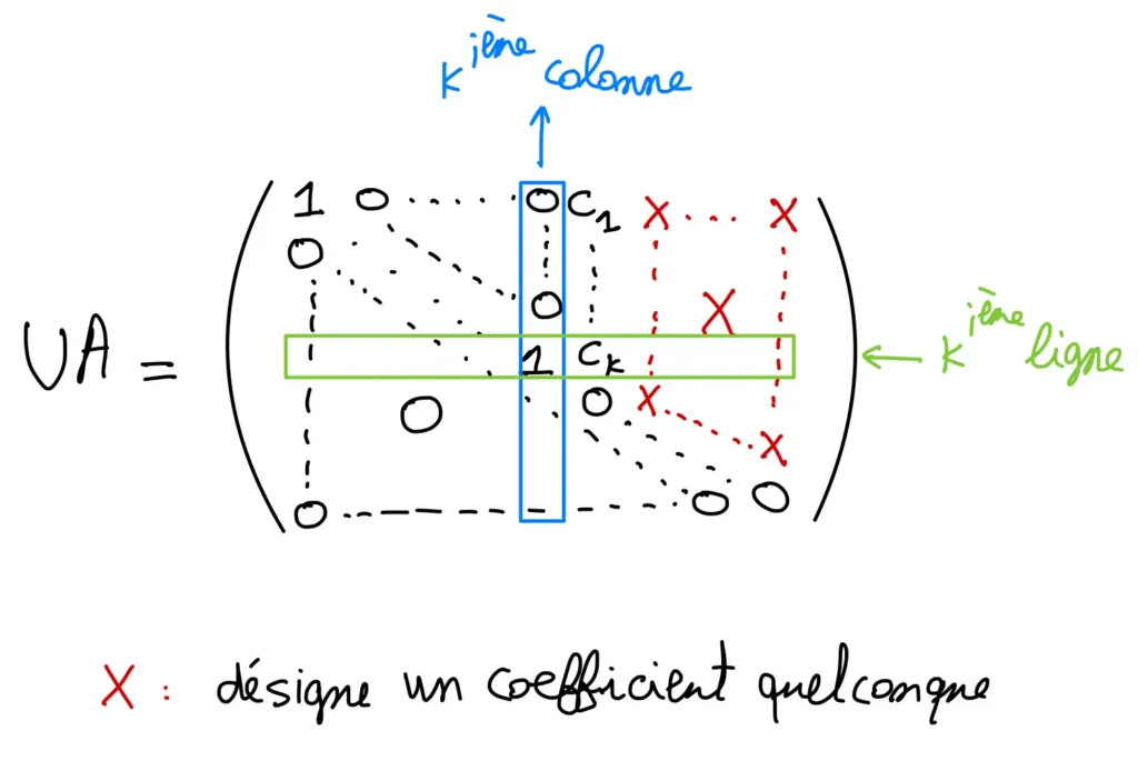
On pose X=\begin{pmatrix}-c_{1} \\ \vdots \\ -c_{k} \\ 1 \\ \vdots \\ 0\end{pmatrix}.
On a U A X=0, bien que X \neq 0.
Il en résulte que la matrice UA n'est pas inversible.
Or U est inversible car c'est un produit de matrices d'opérations élémentaires. On déduit alors que A n'est pas inversible. Par contraposée, on conclut que si A est inversible alors tous les coefficients diagonaux de A sont nuls.
Exemple 13 :
i) La matrice \begin{pmatrix}1 & 1 & 1 \\ 0 & 0 & 1 \\ 0 & 0 & -1\end{pmatrix} n'est pas inversible.
ii) La matrice \begin{pmatrix}1 & 0 & 0 \\ 1 & 2 & 0 \\ 0 & 0 & -1\end{pmatrix} est inversible.
iii) Pour tout \left(\lambda_{1}, \ldots, \lambda_{n}\right) de \mathbb{K}^{*^{n}} la matrice diag \left(\lambda_{1}, \ldots, \lambda_{n}\right) est inversible et son inverse est diag \left(\lambda_{1}^{-1}, \ldots, \lambda_{n}^{-1}\right).